
In the previous section, the f-chart method is presented. Due to the limitations outlined in Section 11.1.5, the f-chart method cannot be used for systems in which the minimum temperature supplied to a load is not near 20 °C. Most of the systems that cannot be simulated with f-chart can be modeled with the utilizability method or its enhancements.
The utilizability method is a design technique used for the calculation of the long-term thermal collector performance for certain types of systems. Initially originated by Whillier (1953), the method, referred to as the Ф-curve method, is based on the solar radiation statistic, and the necessary calculations have to be done at hourly intervals about solar noon each month. Subsequently, the method was generalized for the time of year and geographic location by Liu and Jordan (1963). Their generalized Φ-curves, generated from daily data, gave the ability to calculate utilizability curves for any location and tilt by knowing only the clearness index, KT. Afterward, the work by Klein (1978) and Collares-Pereira and Rabl (1979a) eliminated the necessity of hourly calculations. The monthly average daily utilizability, ![]() reduced much of the complexity and improved the utility of the method.
reduced much of the complexity and improved the utility of the method.
11.2.1 Hourly utilizability
The utilizability method is based on the concept that only radiation that is above a critical or threshold intensity is useful. Utilizability, Φ, is defined as the fraction of insolation incident on a collector’s surface that is above a given threshold or critical value.
We saw in Chapter 3, Section 3.3.4, Eq. (3.61), that a solar collector can give useful heat only if solar radiation is above a critical level. When radiation is incident on the tilted surface of a collector, the utilizable energy for any hour is (It − Itc)+, where the plus sign indicates that this energy can be only positive or zero. The fraction of the total energy for the hour that is above the critical level is called the utilizability for that hour, given by:
![]() (11.43)
(11.43)
Utilizability can also be defined in terms of rates, using Gt and Gtc, but because radiation data are usually available on an hourly basis, the hourly values are preferred and are also in agreement with the basis of the method.
Utilizability for a single hour is not very useful, whereas utilizability for a particular hour of a month having N days, in which the average radiation for the hour is ![]() is very useful, given by:
is very useful, given by:
![]() (11.44)
(11.44)
In this case, the average utilizable energy for the month is given by ![]() Such calculations can be done for all hours of the month, and the results can be added up to get the utilizable energy of the month. Another required parameter is the dimensionless critical radiation level, defined as:
Such calculations can be done for all hours of the month, and the results can be added up to get the utilizable energy of the month. Another required parameter is the dimensionless critical radiation level, defined as:
![]() (11.45)
(11.45)
For each hour or hour pair, the monthly average hourly radiation incident on the collector is given by:
![]() (11.46)
(11.46)
Dividing by ![]() and using Eq. (2.82a),
and using Eq. (2.82a),
![]() (11.47)
(11.47)
The ratios r and rd can be estimated from Eqs. (2.83) and (2.84), respectively.
Liu and Jordan (1963) constructed a set of Ф curves for various values of ![]() With these curves, it is possible to predict the utilizable energy at a constant critical level by knowing only the long-term average radiation. Later on Clark et al. (1983) developed a simple procedure to estimate the generalized Ф functions, given by:
With these curves, it is possible to predict the utilizable energy at a constant critical level by knowing only the long-term average radiation. Later on Clark et al. (1983) developed a simple procedure to estimate the generalized Ф functions, given by:
 (11.48a)
![]() (11.48b)
(11.48b)
![]() (11.48c)
(11.48c)
The monthly average hourly clearness index, ![]() based on Eq. (2.82c), is given by:
based on Eq. (2.82c), is given by:
![]() (11.49)
(11.49)
and can be estimated using Eqs (2.83) and (2.84) as:
![]() (11.50)
(11.50)
where α and β can be estimated from Eqs (2.84b) and (2.84c), respectively. If necessary, ![]() can be estimated from Eq. (2.79) or obtained directly from Table 2.5.
can be estimated from Eq. (2.79) or obtained directly from Table 2.5.
The ratio of monthly average hourly radiation on a tilted surface to that on a horizontal surface, ![]() is given by:
is given by:
![]() (11.51)
(11.51)
The Ф curves are used hourly, which means that three to six hourly calculations are required per month if hour pairs are used. For surfaces facing the equator, where hour pairs can be used, the monthly average daily utilizability, ![]() presented in the following section can be used and is a more simple way of calculating the useful energy. For surfaces that do not face the equator or for processes that have critical radiation levels that vary consistently during the days of a month, however, the hourly Ф curves need to be used for each hour.
presented in the following section can be used and is a more simple way of calculating the useful energy. For surfaces that do not face the equator or for processes that have critical radiation levels that vary consistently during the days of a month, however, the hourly Ф curves need to be used for each hour.
11.2.2 Daily utilizability
As can be understood from the preceding description, a large number of calculations are required to use the Ф curves. For this reason, Klein (1978) developed the monthly average daily utilizability, ![]() concept. Daily utilizability is defined as the sum over all hours and days of a month of the radiation falling on a titled surface that is above a given threshold or critical value, which is similar to the one used in the Ф concept, divided by the monthly radiation, given by:
concept. Daily utilizability is defined as the sum over all hours and days of a month of the radiation falling on a titled surface that is above a given threshold or critical value, which is similar to the one used in the Ф concept, divided by the monthly radiation, given by:
![]() (11.52)
(11.52)
The monthly utilizable energy is then given by the product ![]() . The value of
. The value of ![]() for a month depends on the distribution of hourly values of radiation in that month. Klein (1978) assumed that all days are symmetrical about solar noon, and this means that
for a month depends on the distribution of hourly values of radiation in that month. Klein (1978) assumed that all days are symmetrical about solar noon, and this means that ![]() depends on the distribution of daily total radiation, i.e., the relative frequency of occurrence of below-average, average, and above-average daily radiation values. In fact, because of this assumption, any departure from this symmetry within days leads to increased values of
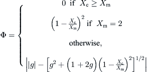
depends on the distribution of daily total radiation, i.e., the relative frequency of occurrence of below-average, average, and above-average daily radiation values. In fact, because of this assumption, any departure from this symmetry within days leads to increased values of ![]() . This means that the
. This means that the ![]() calculated gives conservative results.
calculated gives conservative results.
Klein developed the correlations of ![]() as a function of
as a function of ![]() , a dimensionless critical radiation level,
, a dimensionless critical radiation level, ![]() and a geometric factor
and a geometric factor ![]() . The parameter
. The parameter ![]() is the monthly ratio of radiation on a tilted surface to that on a horizontal surface,
is the monthly ratio of radiation on a tilted surface to that on a horizontal surface, ![]() given by Eq. (2.107), and Rn is the ratio for the hour centered at noon of radiation on the tilted surface to that on a horizontal surface for an average day of the month, which is similar to Eq. (2.99) but rewritten for the noon hour in terms of rdHD and rH as:
given by Eq. (2.107), and Rn is the ratio for the hour centered at noon of radiation on the tilted surface to that on a horizontal surface for an average day of the month, which is similar to Eq. (2.99) but rewritten for the noon hour in terms of rdHD and rH as:
![]() (11.53)
(11.53)
where rd,n and rn are obtained from Eqs (2.83) and (2.84), respectively, at solar noon (h = 0°). It should be noted that Rn is calculated for a day that has a total radiation equal to the monthly average daily total radiation, i.e., a day for which ![]() and Rn is not the monthly average value of R at noon. The term HD/H is given from Erbs et al. (1982) as follows.
and Rn is not the monthly average value of R at noon. The term HD/H is given from Erbs et al. (1982) as follows.
For hss ≤ 81.4°,
![]() (11.54a)
(11.54a)
For hss > 81.4°,
![]() (11.54b)
(11.54b)
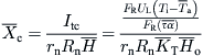
The monthly average critical radiation level, ![]() is defined as the ratio of the critical radiation level to the noon radiation level on a day of the month in which the radiation is the same as the monthly average, given by:
is defined as the ratio of the critical radiation level to the noon radiation level on a day of the month in which the radiation is the same as the monthly average, given by:
![]() (11.55)
(11.55)
The procedure followed by Klein (1978) was that, for a given ![]() a set of days was established that had the correct long-term average distribution of KT values. The radiation in each of the days in a sequence was divided into hours, and these hourly values of radiation were used to find the total hourly radiation on a tilted surface, It. Subsequently, critical radiation levels were subtracted from the It values and summed as shown in Eq. (11.52) to get the
a set of days was established that had the correct long-term average distribution of KT values. The radiation in each of the days in a sequence was divided into hours, and these hourly values of radiation were used to find the total hourly radiation on a tilted surface, It. Subsequently, critical radiation levels were subtracted from the It values and summed as shown in Eq. (11.52) to get the ![]() values. The
values. The ![]() curves calculated in this manner can be obtained from graphs or the following relation:
curves calculated in this manner can be obtained from graphs or the following relation:
![]() (11.56a)
(11.56a)
where
![]() (11.56b)
(11.56b)
![]() (11.56c)
(11.56c)
![]() (11.56d)
(11.56d)
EXAMPLE 11.11
A north-facing surface located in an area that is at 35°S latitude is tilted at 40°. For the month of April, when ![]() = 17.56 MJ/m2, critical radiation is 117 W/m2, and ρG = 0.25, calculate
= 17.56 MJ/m2, critical radiation is 117 W/m2, and ρG = 0.25, calculate ![]() and the utilizable energy.
and the utilizable energy.
Solution
For April, the mean day from Table 2.1 is N = 105 and δ = 9.41°. From Eq. (2.15), the sunset time hss = 83.3°. From Eqs (2.84b), (2.84c), and (2.84a), we have:


From Eq. (2.83), we have:

From Eq. (2.90a), for the Southern Hemisphere (plus sign instead of minus),

From Eq. (2.79) or Table 2.5, Ho = 24.84 kJ/m2, and from Eq. (2.82a),
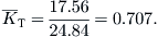
For a day in which ![]() KT = 0.707, and from Eq. (11.54b),
KT = 0.707, and from Eq. (11.54b),

Then, from Eq. (11.53),
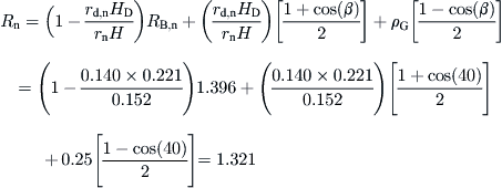
From Eq. (2.109), for the Southern Hemisphere (plus sign instead of minus),

From Eq. (2.108), for the Southern Hemisphere (plus sign instead of minus),
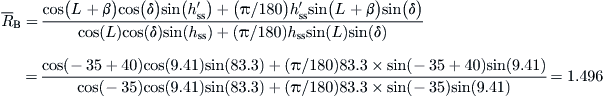
From Eq. (2.105d),

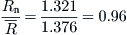
From Eq. (2.107),
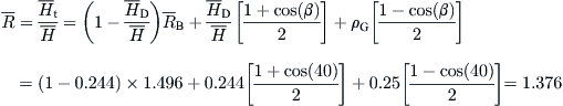
Now,
From Eq. (11.55), the dimensionless average critical radiation level is:
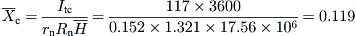
From Eq. (11.56):


Finally, the month utilizable energy is:

Both the Ф and the ![]() concepts can be applied in a variety of design problems, such as heating systems and passively heated buildings, where the unutilizable energy (excess energy) that cannot be stored in the building mass can be estimated. Examples of these applications are given in the following sections.
concepts can be applied in a variety of design problems, such as heating systems and passively heated buildings, where the unutilizable energy (excess energy) that cannot be stored in the building mass can be estimated. Examples of these applications are given in the following sections.
11.2.3 Design of active systems with the utilizability method
The method can be developed for an hourly or daily basis. These are treated separately in this section.
Hourly utilizability
Utilizability can also be defined as the fraction of incident solar radiation that can be converted into a useful heat. It is the fraction utilized by a collector having no optical losses and a heat removal factor of unity, i.e., FR(τα) = 1, operating at a fixed inlet to ambient temperature difference. It should be noted that the utilizability of this collector is always less than 1, since thermal losses exist in the collector.
The Hottel–Whillier equation (Hottel and Whillier, 1955) relates the rate of useful energy collection by a flat-plate solar collector, Qu, to the design parameters of the collector and meteorological conditions. This is given by Eq. (3.60) in Chapter 3, Section 3.3.4. This equation can be expressed in terms of the hourly radiation incident on the collector plane, It, as:
![]() (11.57)
(11.57)
FR = collector heat removal factor;
(τα) = effective transmittance–absorptance product;
It = total radiation incident on the collector surface per unit area (kJ/m2);
UL = energy loss coefficient (kJ/m2 K);
Ti = inlet collector fluid temperature (°C); and
Ta = ambient temperature (°C).
The radiation level must exceed a critical value before useful output is produced. This critical level is found by setting Qu in Eq. (11.57) equal to 0. This is given in Eq. (3.61), but in terms of the hourly radiation incident on the collector plane, it is given by:
![]() (11.58)
(11.58)
The useful energy gain can thus be written in terms of critical radiation level as:
![]() (11.59)
(11.59)
The plus superscript in Eqs (11.57) and (11.59) and in the following equations indicates that only positive values of Itc are considered. If the critical radiation level is constant for a particular hour of the month having N days, then the monthly average hourly output for this hour is:
![]() (11.60)
(11.60)
Because the monthly average radiation for this particular hour is ![]() the average useful output can be expressed by:
the average useful output can be expressed by:
![]() (11.61)
(11.61)
where Ф is given by Eq. (11.44). This can be estimated from the generalized Ф curves or Eq. (11.48), given earlier for the dimensionless critical radiation level, Xc, given by Eq. (11.45), which can now be written in terms of the collector parameters, using Eq. (11.58), as:
![]() (11.62)
(11.62)
where (τα)/(τα)n can be determined for the mean day of the month, shown in Table 2.1, and the appropriate hour angle and can be estimated with the incidence angle modifier constant, bo, from Eq. (4.25).
With Ф known, the utilizable energy is ![]() . The main use of hourly utilizability is to estimate the output of processes that have a critical radiation level, Xc, that changes considerably during the day, which can be due to collector inlet temperature variation.
. The main use of hourly utilizability is to estimate the output of processes that have a critical radiation level, Xc, that changes considerably during the day, which can be due to collector inlet temperature variation.
EXAMPLE 11.12
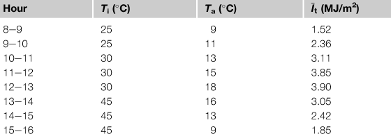
Suppose that a collector system supplies heat to an industrial process. The collector inlet temperature (process return temperature) varies as shown in Table 11.11 but, for a certain hour, is constant during the month. The calculation is done for the month of April, where ![]() The system is located at 35°N latitude and the collector characteristics are FRUL = 5.92 W/m2 °C, FR(τα)n = 0.82, tilted at 40°, and the incidence angle modifier constant bo = 0.1. The weather conditions are also given in the table. Calculate the energy output of the collector.
The system is located at 35°N latitude and the collector characteristics are FRUL = 5.92 W/m2 °C, FR(τα)n = 0.82, tilted at 40°, and the incidence angle modifier constant bo = 0.1. The weather conditions are also given in the table. Calculate the energy output of the collector.
Table 11.11
Collector Inlet Temperature and Weather Conditions for Example 11.12
Solution
First, the incidence angle is calculated, from which the incidence angle modifier is estimated. The estimations are done on the half hour; for the hour 8–9, the hour angle is −52.5°. From Eq. (2.20),

From Eq. (4.25),

The dimensionless critical radiation level, Xc, is given by Eq. (11.62):
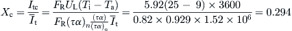
From Table 2.5, ![]() From the input data and Eq. (2.82a),
From the input data and Eq. (2.82a),

To avoid repeating the same calculations as in previous examples, some values are given directly. Therefore, hss = 96.7°, α = 0.709, and β = 0.376. From Eq. (2.84a),

From Eq. (2.83), we have:

From Eq. (11.51),
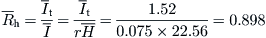
The monthly average hourly clearness index, ![]() is given by Eq. (11.50):
is given by Eq. (11.50):

From Eq. (11.48c),

From Eq. (11.48b),
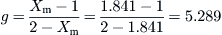
From Eq. (11.48a),

Finally the useful gain (UG) of the collector for that hour is (April has 30 days):

The results for the other hours are shown in Table 11.12.
Table 11.12
Results for All Hours in Example 11.12
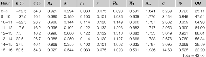
The useful gain for the month is equal to 427.6 MJ/m2.
Although the Ф curves method is a very powerful tool, caution is required to avoid possible misuse. For example, due to finite storage capacity, the critical level of collector inlet temperature for liquid-based domestic solar heating systems varies considerably during the month, so the Ф curves method cannot be applied directly. Exceptions to this rule are air heating systems during winter, where the inlet air temperature to the collector is the return air from the house, and systems with seasonal storage where, due to its size, storage tank temperatures show small variations during the month.
Daily utilizability
As indicated in Section 11.2.2, the use of Ф curves involves a lot of calculations. Klein (1978) and Collares-Pereira and Rabl (1979b, c) simplified the calculations for systems for which a critical radiation level can be used for all hours of the month.
Daily utilizability is defined as the sum for a month over all hours and all days of the radiation on a tilted surface that is above a critical level, divided by the monthly radiation. This is given in Eq. (11.52). The critical level, Itc, is similar to Eq. (11.58), but in this case, the monthly average (τα) product must be used and the inlet and ambient temperatures are representative temperatures for the month:
![]() (11.63)
(11.63)
In Eq. (11.63), the term ![]() can be estimated with Eq. (11.11). The monthly average critical radiation ratio is the ratio of the critical radiation level, Itc, to the noon radiation level for a day of the month in which the total radiation for the day is the same as the monthly average. In equation form,
can be estimated with Eq. (11.11). The monthly average critical radiation ratio is the ratio of the critical radiation level, Itc, to the noon radiation level for a day of the month in which the total radiation for the day is the same as the monthly average. In equation form,
 (11.64)
The monthly average daily useful energy gain is given by:
![]() (11.65)
(11.65)
Daily utilizability can be obtained from Eq. (11.56).
It should be noted that, even though monthly average daily utilizability reduces the complexity of the method, calculations can be still quite tedious, especially when monthly average hourly calculations are required.
It is also noticeable that the majority of the aforementioned methods for computing solar energy utilizability have been derived as fits to North American data versus the clearness index, which is the parameter used to indicate the dependence of the climate. Carvalho and Bourges (1985) applied some of these methods to European and African locations and compared results with values obtained from long-term measurements. Results showed that these methods can give acceptable results when the actual monthly average daily irradiation on the considered surface is known.
Examples of this method are given in the next section, where the ![]() and f-chart methods are combined.
and f-chart methods are combined.
Leave a Reply