TRANSFORMER ON LOAD

When a certain load is connected across the secondary, a current I₂ flows through it as shown in Figure 10.16. The magnitude of current I₂ depends upon terminal voltage V₂ and impedance of the load. The phase angle of secondary current I₂ with respect to V₂ depends upon the nature of load, that is, whether the load is resistive, inductive, or capacitive.

(Neglecting winding resistance and leakage flux)

When a certain load is connected across the secondary, a current I₂ flows through it as shown in Figure 10.16. The magnitude of current I₂ depends upon terminal voltage V₂ and impedance of the load. The phase angle of secondary current I₂ with respect to V₂ depends upon the nature of load, that is, whether the load is resistive, inductive, or capacitive.

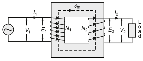
Fig. 10.16  Transformer on load

The operation of the transformer on load is explained below with the help of number of diagrams:

1. When the transformer is on no-load as shown in Figure 10.17(a), it draws no-load current I₀ from the supply mains. The no-load current I₀ produces an mmf. N₁I₀ which sets up flux in the core.
2. When the transformer is loaded, current I₂ flows in the secondary winding. This secondary current I₂ produces an mmf N₂I₂ which sets up flux ɸ₂ in the core. This flux opposes the flux which is set up by the current I₀ as shown in Figure 10.17(b), according to Lenz’s law.
3. Since ɸ₂ opposes the flux, and therefore, the resultant flux tends to decrease and causes the reduction of self-induced emf E₁ momentarily. Thus, V₁ predominates over E₁ causing additional primary current  drawn from the supply mains. The amount of this additional current is such that the original conditions, that is, flux in the core must be restored to original value ɸ, so that V₁ = E₁. The current I₁ is in phase opposition with I₂ and is called primary counterbalancing current. This additional current  produces an mmf N₁ which sets up flux, ɸ, in the same direction as that of ɸ as shown in Figure 10.17(c) and cancels the flux ɸ₂ set up by mmf N₂I₂.Now, N₁ = N₂I₂ (ampere-turns balance)∴
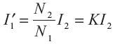
4. Thus, the flux is restored to its original value as shown in Figure 10.17(d). The total primary current I₁ is the vector sum of current I₀ and I′, that is, I₁ = I₀+ .

This shows that flux in the core of a transformer remains the same from no-load to full load; this is the reason why iron losses in a transformer remain the same from no-load to full load

Fig. 10.17  (a), (b), (c) and (d) : Effect on the magnetic flux set-up in the core when transformer is loaded

10.10  PHASOR DIAGRAM OF A LOADED TRANSFORMER

(Neglecting voltage drops in the winding; ampere-turns balance)

Since the voltage drops in both the windings of the transformer are neglected,

 

V₁ = E₁ and E₂ = V₂

While drawing the phasor diagram, the following important points are to be considered.

1. For simplicity, let the transformation ratio K = l be considered, and therefore, E₂ = E₁.
2. The secondary current I₂ is in phase, lags behind, and leads the secondary terminal voltage V₂ by an angle ɸ₂ for resistive, inductive, and capacitive load, respectively.
3. The counterbalancing current (i.e.,  = KI₂ here K = 1 ∴  = I₂) and is 180° out of phase with I₂.
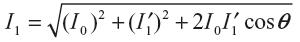
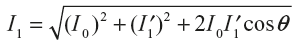
4. The total primary current I₁ is the vector sum of no-load primary current I₀ and counter balancing current That is,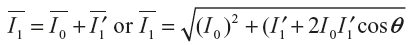Where θ is the phase angle between I₀ and 
5. The p.f. on the primary side is cos ɸ₁ which is less than the load p.f. cos ɸ₂ on the secondary side. Its value is determined by the relation. 

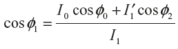
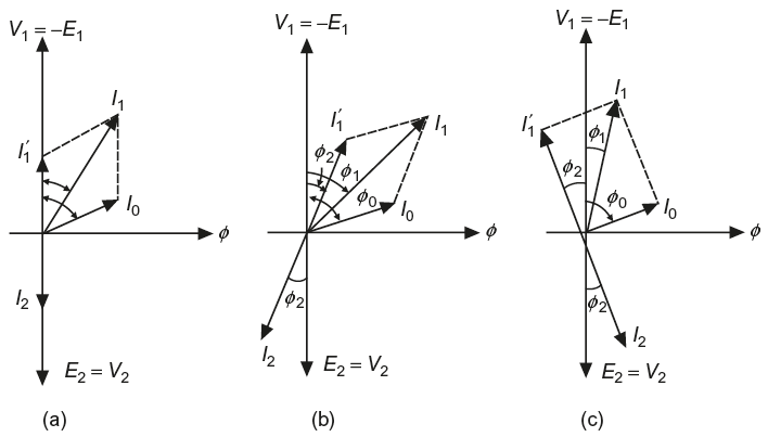
Fig. 10.18  Phasor diagram (a) for resistive load (b) for inductive load (c) for capacitive load

The phasor diagrams of the transformer for resistance, inductive, and capacitive loads are shown in Figure 10.18(a), (b), and (c), respectively.

Alternately,

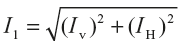
The primary current I₁ can also be determined by resolving the vectors, that is,

 

I_v = I₀ cos ɸ₀ +  cosɸ₂ [where sin ɸ₀ = sincos⁻¹(cos ɸ₀)

I_H = I₀ sin ɸ₀ +  sin ɸ₂ and sin ɸ₂ = sincos⁻¹(cos ɸ₂)]

Example 10.12

A single-phase transformer with a ratio of 440/110 V takes a no-load current of 5 A at 0.2 p.f. lagging. If the secondary supplies a current of 120 A at p.f. of 0.8 lagging, calculate the primary current and p.f.

Solution:

Transformation ratio,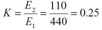 

Let the primary counterbalancing current be 

Then,

 = KI₂ = 0.25 × 120 =30A

Now,

 

cos ɸ₀ = 0.2; ɸ₀ = cos⁻¹0.2 = 78.46°

cos ɸ₂ = 0.8; ɸ₂ = cos⁻¹0.8 = 36.87°

θ = ɸ₀ − ɸ₂ = 78.46° − 36.87° = 41.59°

Primary p.f.,

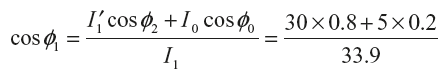
= 0.7375 lag

Example 10.13

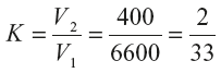
A single-phase transformer with a ratio of 6600/400 V (primary to secondary voltage) takes to no-load current of 0.7 A at 0.24 power factor lagging. If the secondary winding supplies a current of 120 A at a power factor of 0.8 lagging. Estimate the current drawn by the primary winding.

Solution:

Here,

 

I₀ = 0.7 A; cos ɸ₀ = 0.24 lag; I₂ = 120 A; cos ɸ₂ = 0.8 lag

Transformation ratio,

Let the primary counterbalance current be I₁.

∴

N₁ = N₂I₂

or

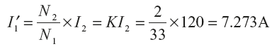
Now,

 

cos ɸ₀ = 0.24; ɸ₀ = cos⁻¹0.24 = 76.11°

cos ɸ₂ = 0.8; ɸ₂ = cos⁻¹0.8 = 36.87°

Angle between vector I₀ and I₁ (Figure 10.14(b))

 

θ = 76.11° − 36.87° = 39.24°

Current drawn by the primary,